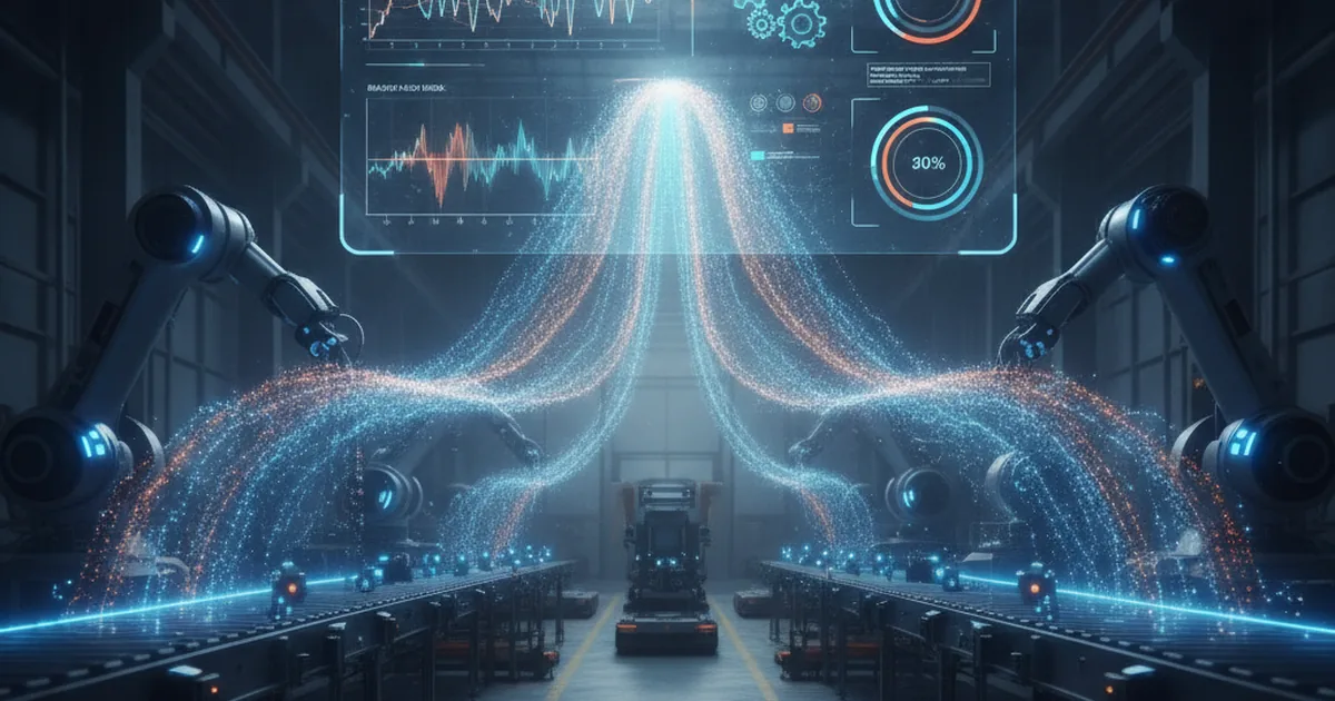
Unplanned downtime costs automotive manufacturers an average of $250,000 per hour — a figure that climbs to over $500,000 per hour in semiconductor fabrication. Traditional scheduled maintenance is a statistical guess: replace bearings every 6 months regardless of actual condition, and you will replace components that had months of life left while still being blindsided by the bearing that failed at month five. Condition monitoring closed part of that gap by watching individual sensor thresholds, but it fires an alert at the moment a problem emerges — often too late to avoid a production stop. Digital twins take a fundamentally different approach: they model the entire asset as a system, track its degradation trajectory in real time, and tell maintenance teams days or weeks in advance that a failure is coming. The data flows through a coherent IIoT architecture from sensor to prediction engine, turning raw signals into actionable schedules.
TL;DR
A digital twin continuously mirrors your physical asset using live sensor data and ML models, enabling maintenance teams to predict failures days or weeks ahead — not react to them. This guide covers how the technology works, a five-step implementation path, common pitfalls, and the ROI metrics manufacturers actually measure.
Making those predictions useful on the plant floor means getting the right alert to the right person at the right time. Field engineers need to receive remaining useful life (RUL) estimates and generated work orders through industrial mobile applications — custom interfaces designed for shop-floor conditions, not desktop ERP portals — often the most direct ROI multiplier in the first deployment year.
What Is a Digital Twin in Predictive Maintenance?
A digital twin is a continuously updated virtual replica of a physical asset, synchronized in real time with live sensor data from the machine it represents. It is not a static 3D CAD model, a visualization dashboard, or a SCADA screen. The distinction matters: a CAD model or dashboard reflects engineering intent or current sensor readings, while a digital twin runs behavioral models — physics-based simulations, machine learning algorithms, or hybrids — that forecast how the asset will behave and degrade over time.
In a predictive maintenance context, the twin's primary output is a failure probability curve and a Remaining Useful Life (RUL) estimate: how many operating hours, cycles, or calendar days remain before the asset will cross a defined degradation threshold. That number, updated continuously, is what drives just-in-time maintenance scheduling.
The Four Maturity Levels of Industrial Digital Twins
Industrial digital twin implementations span a wide range of sophistication. A useful framework organizes them into four levels:
| Level | Name | Capability |
|---|---|---|
| 1 | Descriptive | Static model, manual data entry; essentially a digital record of the asset's design specs and maintenance history |
| 2 | Informative | Real-time sensor feeds connected; provides current-state visibility — what the machine is doing right now |
| 3 | Predictive | ML or physics-based models running on live data; produces RUL forecasts and failure probability scores |
| 4 | Autonomous | Closed-loop: the twin's predictions automatically trigger CMMS work orders, parts reservations, and technician dispatch without human intervention |
Most manufacturers beginning their digital twin journey start at Level 2 — connecting sensors is a solved problem; it is the cheapest way to prove value quickly. Level 3 is the sweet spot for predictive maintenance ROI: you gain the forecasting capability without the organizational complexity of fully autonomous dispatch. Level 4 requires months of model validation and high technician trust before it is safe to automate work-order generation.
Digital Twin vs. Traditional Condition Monitoring
Traditional condition monitoring sets static alarm thresholds on individual sensor channels: if bearing temperature exceeds 85°C, fire an alert. A digital twin integrates dozens of sensor streams into a behavioral model of the whole asset, tracks how the pattern of signals deviates from healthy baseline over time, and produces a failure probability timeline — not a binary "alarm / no alarm" decision at the instant the threshold is crossed.
How the Data Flow Works — From Sensor to Prediction
Understanding the data pipeline is essential for both engineers evaluating the technology and teams scoping the implementation effort. The chain has three distinct stages: sensing, modeling, and acting.
The Sensor Layer
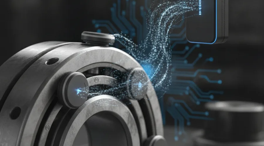
The sensor selection for any digital twin should be driven by the asset's Failure Mode and Effects Analysis (FMEA) output, not by what is easy to install. That said, a minimum viable sensor set for rotating machinery — the category covering motors, pumps, compressors, turbines, gearboxes — consists of:
- Triaxial vibration (MEMS accelerometer): detects imbalance, misalignment, looseness, and bearing defects through frequency analysis
- Bearing temperature (RTD or thermocouple): rising temperature under load is an early indicator of lubrication breakdown
- Motor current (current transformer): current signature analysis can detect rotor bar cracks, air-gap eccentricity, and load anomalies without contact with the rotating element
- Shaft speed (encoder or tachometer): required to normalize vibration features against RPM; critical for assets running at variable speed
High-value secondary sensors — pressure, flow, acoustic emission, oil-analysis inline sensors — add failure mode coverage that the core four cannot provide. For a compressor stage, differential pressure and outlet temperature add thermodynamic efficiency indicators that track valve wear invisible to vibration alone.
Physics-Based Models vs. ML Models
Once sensor data is flowing, the modeling approach determines both the accuracy ceiling and the implementation timeline:
- Physics-based (first-principles / finite element): encodes the mechanical or thermodynamic laws governing the asset's behavior. High accuracy on known failure modes, interpretable outputs, and no historical failure data required to start. The trade-off: requires deep domain engineering knowledge to build and is asset-specific — a model built for a 200kW centrifugal pump does not transfer to a 500kW axial pump without re-engineering.
- ML-based (LSTM recurrent networks, gradient boosting, Gaussian process regression): learns degradation patterns from historical run-to-failure data. Faster to deploy when that data exists, generalizes across asset variants, and improves automatically as more failure events are recorded. Limitation: requires meaningful failure history; a machine with only three historical failures provides too little signal for a data-hungry deep network.
- Hybrid (physics-informed ML): the physics model provides the feature space — extracting thermodynamic efficiency coefficients, calculating bearing defect frequencies from FMEA output — while an ML layer learns the residual patterns that pure physics cannot capture. This is industry best practice for critical assets where both interpretability and adaptability matter.
Remaining Useful Life (RUL) Calculation
RUL is the operational metric that connects raw sensor signals to a scheduling decision. Conceptually, the calculation follows a five-step chain:
- Raw signal ingestion: time-series sensor data streamed at 1–10 kHz for vibration, 1–60 Hz for temperature and process variables
- Feature extraction: compute statistical features per sampling window — RMS vibration amplitude, kurtosis (impulsiveness indicator for bearing pitting), temperature delta from baseline, frequency-domain energy in bearing defect frequency bands
- Degradation index construction: combine features into a single monotonic health score that moves from 1.0 (healthy) toward 0 (failure threshold) as the asset degrades
- Survival model / regression: fit a model that maps the current degradation index trajectory to a probability distribution over time-to-failure
- RUL estimate output: the median of that distribution (with a confidence interval) is the RUL number surfaced to the maintenance team
Maintenance teams need a number, not a probability distribution lecture. "Bearing #3 on Compressor C7: RUL = 18 days (80% confidence interval: 11–26 days)" is actionable. A raw probability curve is not. The CMMS integration in Step 4 of implementation translates the RUL number into a work order priority and lead time.
Reactive vs. Preventive vs. Predictive — A Maintenance Strategy Comparison
Choosing where to apply digital twin technology requires a clear-eyed comparison of the three dominant maintenance strategies and their cost profiles:
| Dimension | Reactive | Preventive (time-based) | Predictive (digital twin) |
|---|---|---|---|
| When action triggers | After failure | Fixed calendar interval | Condition-based, failure forecast |
| Downtime type | Unplanned (longest) | Planned (sometimes unnecessary) | Planned (minimal, just-in-time) |
| Parts usage | Emergency stock, premium cost | Over-replacement common | Replaced at end of useful life |
| Data required | None | MTBF history | Live sensors + ML model |
| Typical cost vs. reactive | Baseline (highest) | −10 to −20 % | −25 to −35 % |
Reactive maintenance is not always wrong. For non-critical assets that are cheap to replace, have no safety consequence on failure, and do not sit on the critical production path — a $200 relay switch, a conveyor belt tensioner — the sensor infrastructure and modeling overhead of a digital twin is not justified. The highest-value targets for digital twin investment are rotating equipment on the critical path where each hour of downtime has a measurable revenue cost, assets with failure modes that develop gradually over weeks, and equipment where parts lead time exceeds the warning window that condition monitoring provides.
Implementing a Digital Twin for Predictive Maintenance — 5 Steps
Most failed digital twin pilots suffer from the same pattern: teams start with the most technically interesting asset, not the one with the largest business case, and they underscope the integration work. A disciplined five-step path avoids both traps.
Step 1: Define Scope and Asset Criticality
Before selecting any technology, rank candidate assets using a criticality matrix that scores each machine on three dimensions: consequence of failure (production impact, safety exposure, regulatory risk), probability of failure (historical MTBF, age, operating stress), and maintenance cost (emergency repair cost vs. planned intervention cost). Multiply the three scores and rank the result. Start the pilot on the top 3–5 assets by that composite score — not the newest machines, not the ones with the most available data, but the ones where predictive capability has the highest financial value. This discipline is what turns a pilot into a business case that funds the next phase.
Step 2: Deploy the Sensor Layer
For legacy OT equipment without native digital outputs, the path to sensor connectivity is wireless retrofit: MEMS vibration nodes and temperature transmitters that clamp onto bearing housings, an industrial edge gateway that aggregates their readings, and OPC UA or MQTT for secure northbound transport to the modeling platform. A basic wireless sensor kit for one rotating asset runs $500–$2,000 in hardware; no PLC modification or process interruption is required for installation. Protocol translation — Modbus RTU from legacy PLCs, PROFINET from servo drives, raw analog from temperature transmitters — is handled at the gateway, not in the cloud model.
Step 3: Collect Baseline Data and Build the Model
Resist the urge to deploy the prediction model before you have baseline data. A minimum of 4–6 weeks of continuous recording under normal operating conditions is required before any ML model can distinguish anomaly from normal variation. Use this window to verify sensor data quality, identify and correct installation problems (a loosely mounted accelerometer introduces its own vibration signature), and collect operational context — speed setpoints, load profiles, product changeovers — that the model needs as conditioning variables. Where historical maintenance records exist with timestamped failure events, use them for supervised training; even five labeled failure records improve a model's failure-mode specificity substantially. Physics-based models can start from day one, using known bearing geometry and material properties, but they still benefit from a baseline period for thermal calibration.
Step 4: Integrate with CMMS/MES
A digital twin that generates predictions without acting on them is a monitoring dashboard with extra steps. The business value is realized when an RUL crossing a threshold automatically creates a work order in the CMMS, pre-reserves the required parts from inventory, and schedules technician labor — all before the failure occurs. This integration is where most implementations stall, because OT and IT systems rarely speak the same data format. Common integration targets include SAP PM (ISO 15926 data model), IBM Maximo (JSON REST API), and eMaint (native REST). Map the RUL threshold to a work order priority level: RUL > 21 days → informational, 7–21 days → plan this week, < 7 days → urgent dispatch. The parts pre-staging logic — what SKUs, what quantities — should be driven by the FMEA output from Step 1.
Step 5: Close the Feedback Loop
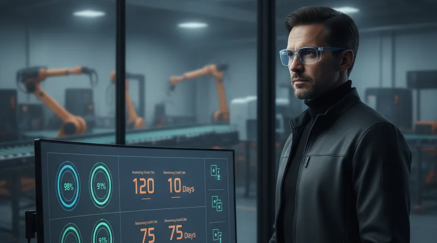
After each maintenance intervention, record whether the predicted failure actually occurred, what the actual condition of the replaced component was, and how far in advance the model flagged it. Feed this labeled data back into the model retraining pipeline. Track three model health KPIs continuously: prediction lead time (average days of advance warning before actual failure), false positive rate (work orders dispatched where the component was found in acceptable condition — keep below 10% to maintain technician trust), and missed failure rate (failures that occurred without a prior prediction — the hardest metric to minimize). A model that generates too many false positives loses operator confidence within weeks; one that misses failures loses the business case. Both must be tracked and the threshold tuned accordingly.
Common Challenges and How to Overcome Them
Legacy Equipment With No Native Connectivity
The single most common objection to digital twin adoption is "our equipment is too old." In practice, roughly 70% of industrial digital twin deployments begin on equipment that predates IIoT by 10–20 years (Systematic Review of Digital Twin-Driven Predictive Maintenance, arXiv 2509.24443, Sep 2026). The path is well-established: wireless retrofit sensor nodes require no electrical work beyond a clamp-on current transformer or a surface-mount temperature patch; they communicate to a DIN-rail-mounted edge gateway over sub-GHz RF or Wi-Fi that does not touch the machine's existing control network. The PLC program is untouched. Protocol translation at the gateway — Modbus RTU → MQTT, serial RS-232 → OPC UA — handles the northbound connection to the digital twin platform. A complete retrofit kit for one motor-pump set, including sensors, gateway, and 12 months of SaaS platform access, typically costs less than one unplanned failure event.
Data Quality and Sensor Noise
A digital twin model is only as good as the data it ingests. Two noise sources systematically degrade model quality and drive false positive rates up. First, structural vibration: a loosely mounted accelerometer picks up building vibration, nearby machine resonances, and its own mounting resonance in addition to the signal of interest. Signal conditioning before model ingestion — a high-pass filter to remove shaft rotation fundamental, a notch filter at building resonance frequency — removes this interference. Second, thermal noise on temperature sensors: raw thermocouple readings can swing ±3°C from electrical interference on a busy plant floor. An exponential moving average with a 60-second window removes this noise while preserving the slow thermal trends relevant to lubrication health. A model fed unfiltered noisy data will produce false-positive rates above 30% within weeks; filtered data consistently achieves rates below 10% (PMC 11054335, Distributed Digital Twin Framework for Predictive Maintenance in IIoT).
Organizational Change Management
The non-technical challenge that kills more digital twin programs than any sensor or software failure: getting maintenance technicians who have built 20 years of schedule-based intuition to trust algorithm-generated work orders. The most effective approach is a two-phase rollout. In Phase 1 (months 1–3), the digital twin operates in advisory mode: predictions are displayed alongside traditional schedule-based work orders, but technicians retain full authority to override or defer. This period generates the accuracy track record — and the conversation. When a technician sees the model flag a bearing 18 days before he would have scheduled the monthly round, and finds the inner race cracking on inspection, trust compounds quickly. In Phase 2 (months 4+), work orders below a criticality threshold are auto-dispatched; critical assets remain advisory until the false-positive rate has been below 10% for 90 consecutive days. Skipping Phase 1 and going straight to autonomous dispatch is the fastest way to get the entire program cancelled after the first erroneous work order.
ROI and KPIs — What to Measure
Leadership approves investment on financial returns; engineering manages the program on operational indicators. Both sets of KPIs are necessary and should be tracked from day one of the pilot.
Financial KPIs
- Unplanned downtime cost per year: baseline this before deployment (hours × hourly cost of downtime) and compare quarterly post-deployment
- Maintenance cost per production unit: normalizes for volume changes; tracks whether labor and parts spend per unit is declining
- Emergency parts spend vs. planned parts spend ratio: the shift from emergency procurement (premium pricing, expediting fees) to planned procurement is often the fastest financial signal
- Asset replacement capex deferred: a 10–15% extension in asset lifespan delays capital replacement; this is often the largest single item in the business case for asset-intensive industries
Operational KPIs
- OEE (Overall Equipment Effectiveness): target +3–5 percentage points from baseline; this captures availability, performance, and quality in a single figure
- MTBF (Mean Time Between Failures): target +20–40% from baseline over 12 months
- MTTR (Mean Time To Repair): target −30%; parts pre-staged before failure dispatch eliminates waiting time from the repair cycle
- Prediction lead time: target ≥7 days average advance warning for critical assets; below 3 days, the maintenance window benefits are minimal
- False positive rate: keep below 10% to maintain technician trust and avoid the program being labeled "the system that cried wolf"
Published Benchmarks
- 20–35% reduction in overall maintenance costs (oxmaint.com 2026; arXiv 2509.24443)
- 40–50% reduction in unplanned downtime (INSIA 2026; PMC 11054335)
- 10–15% extension in asset lifespan
- 12–24 month payback period typical for asset-intensive production lines
These benchmarks come from asset-intensive environments — oil and gas, mining, automotive — where downtime costs are in the high hundreds of thousands per hour. Lighter manufacturing environments will see smaller absolute numbers, but the relative percentage improvements hold across industry sectors.
Need custom digital twin dashboards or IIoT mobile interfaces for your production floor? Explore our industrial mobile application development services →
Frequently Asked Questions
- What is a digital twin in predictive maintenance?
- A digital twin is a continuously updated virtual replica of a physical asset, synchronized with live sensor data. In predictive maintenance it runs physics-based or ML models on that live data to forecast remaining useful life and flag impending failures before they cause downtime.
- How is a digital twin different from traditional condition monitoring?
- Traditional condition monitoring sets static alarm thresholds on individual sensors. A digital twin integrates multi-sensor streams into a model of the whole asset, simulates degradation over time, and produces a failure probability timeline — not just an instantaneous alert.
- What sensors are needed to build a digital twin?
- The minimum viable set for rotating equipment is triaxial vibration, bearing temperature, and motor current. High-value additions include pressure, flow, acoustic emission, and oil-analysis sensors. The exact list depends on the asset's dominant failure modes.
- Can digital twins work with legacy OT equipment?
- Yes, with retrofit sensors and a protocol gateway (OPC UA, MQTT, or Modbus TCP). The digital model does not require the machine to be "smart" — it only needs a sensor layer on top. Roughly 70% of industrial digital twin deployments start on equipment that predates IIoT by 10–20 years.
- What ROI can manufacturers expect from digital twin predictive maintenance?
- Published benchmarks show 20–35% reduction in maintenance costs, 40–50% reduction in unplanned downtime, and 10–15% extension in asset lifespan. Payback periods of 12–24 months are typical for asset-intensive production lines.
- How long does it take to deploy a digital twin for predictive maintenance?
- A pilot covering 3–5 critical assets typically takes 8–16 weeks: 2 weeks for sensor installation and data collection baseline, 4–8 weeks for model training, and 2–4 weeks for CMMS/MES integration and alert tuning. Enterprise-wide rollouts run 6–18 months.
Sources: arXiv 2509.24443, Systematic Review of Digital Twin-Driven Predictive Maintenance in Industrial Engineering (Sep 2026); PMC 11054335, Distributed Digital Twin Framework for Predictive Maintenance in IIoT; ScienceDirect S2405844023017413, Overview of predictive maintenance based on digital twin technology; oxmaint.com, Digital Twins for Maintenance Guide (2026).